
How Much Managed Futures Does a Retirement Portfolio Need?

Updated: 3 days ago
Written by John Macy, Financial Coach, MBA, Retirement Income Certified Professional® (RICP)
Portfolio Diversification Series: Part 1: Portfolio Diversification for Retirement: Why It Matters Part 2: Portfolio Diversification: Building a Truly Diversified Portfolio Part 3: Managed Futures Explained: A Key Portfolio Diversifier Part 4: Best Managed Futures Funds for Retirement Portfolios Part 5: How Much Managed Futures Does A Retirement Portfolio Need? (this article) Part 6: Managed Futures vs. Bonds: Which Diversifier Does Better? |
Introduction
Adding managed futures to a traditional stock-and-bond portfolio can make the portfolio substantially less volatile and reduce its historical peak-to-trough losses. But those benefits come at a price: an allocation that protects a portfolio in difficult markets can also cause it to lag during long stock-market advances.
To find out how much diversification from managed futures may be worthwhile, I tested portfolios that gradually replaced stocks with managed futures in 5-percentage-point increments. I compared both a 75/25 stock/bond portfolio and a conventional 60/40 portfolio over more than 26 years of monthly returns, examining annualized return, volatility, maximum drawdown and risk-adjusted performance.
The results suggest that a relatively small allocation can make a small but measurable difference, while allocations around 30–40% produced a favorable historical balance between return and risk in these tests. But the best allocation depends on the starting portfolio, the market period, and how much return an investor is willing to sacrifice for a smoother ride.
TL;DR — The short version
Adding Managed Futures works, and the benefit is large. Over 26 years, a 40% managed futures allocation cut volatility by 37% and the worst loss from 42% to 16%. The annual return cost averaged just 0.55 points, but that blends a big gain in 2000–2009 with a cost of 3.5 points a year in 2010–2019.
The historical balance point was roughly 30–40% of the total portfolio. In these tests, that range generally offered a favorable balance between annual return and measured risk, replacing about half of the original stock allocation. It is a historical result, not a universal target or a forecast.
It is not free. Over the full 26 years, annual return declined as managed futures were added to the portfolio. The cost is small at first and grows with each addition. Beyond roughly 40–50% (depending on the starting mix), risk starts rising again, so more is not necessarily better.
Results depend heavily on the era. Managed futures boosted returns and cut risk in 2000–2009, cost a lot of return in 2010–2019 (while still reducing risk), and sharply reduced losses in 2020–2026 at a moderate return cost.
Managed Futures are important portfolio diversifiers (especially during more volatile periods) because of their historically low correlation with stocks and bonds. For readers who are unfamiliar with Managed Futures I would recommend reading Managed Futures Explained: A Key Portfolio Diversifier. For readers unfamiliar with the concepts of portfolio diversification I would recommend reading Portfolio Diversification for Retirement: Why It Matters.
Who is this article written for?
This article is written primarily for people who are approaching or already in retirement. I assume that the goal is not to squeeze out the highest possible return from your portfolio. Instead, it is a combination of three things: a respectable return for the amount of risk taken, a ceiling on how bumpy the ride gets (volatility), and a ceiling on how deep the worst decline can be (the maximum drawdown).
Volatility matters more once you are drawing on the portfolio to fund your living expenses. A large decline early in retirement (Sequence of Returns Risk), when you are also taking withdrawals, can do lasting damage because you are selling shares at depressed prices and have fewer shares remaining to recover once the downturn ends. The arithmetic of recovery is unforgiving: a 42% loss needs a 72% gain to get back to even.
So throughout this article we judge managed futures less by whether they raise the portfolio’s return and more by how much risk they remove, and what that costs in reduced return. [Note: This analysis measures historical portfolio returns, volatility and drawdowns; it does not simulate retirement withdrawals or estimate the probability of running out of money. A smaller drawdown may help a retiree who is withdrawing from a portfolio, but the actual effect on retirement sustainability depends on withdrawal rates, spending flexibility, inflation, taxes, and the timing and duration of future market declines.]
What we tested
The starting portfolios. We began with a simple three-fund portfolio: 75% stocks and 25% bonds, with the stock portion split 70/30 between U.S. and international stocks. We used Vanguard Total Stock Market Index Fund (VTSMX), Vanguard Total International Stock Index Fund (VGTSX), and Vanguard Total Bond Market Index Fund (VBMFX). We also repeated the analysis with a 60/40 portfolio, keeping the bond sleeve at 40% and the same 70/30 split within stocks.
The managed futures. Managed futures funds trade futures contracts across stocks, bonds, currencies and commodities. Most follow trends: they buy what has been rising and sell short what has been falling. For most of the analysis that follows we used the SG Trend Index, a benchmark published by Société Générale that equally weights the daily returns of the ten largest trend-following managers that report daily and are open to new investment. Its returns are net of the managers’ fees. It is a benchmark, not a fund you can buy directly. (We test a couple of real funds later.)
The experiment. Starting from each baseline, we moved 5% of the portfolio from stocks into managed futures, measured the results, and repeated (adding additional managed futures in incremental 5% steps) until no stocks were left in the portfolio. Bonds stayed fixed. That produced 16 portfolios from the 75/25 start (0% to 75% managed futures) and 13 from the 60/40 start (0% to 60% managed futures).
The data. Monthly returns from February 2000 through August 2026 (319 months), with monthly rebalancing and no taxes or trading costs. We also split the history into three eras: 2000–2009, 2010–2019, and 2020–2026. These eras included the Tech Stock Bubble bursting, the Great Financial Crisis, COVID, and the dramatic increase in interest rates in 2022, as well as strong market returns from 2010-2019 and from 2023-2026.
The four yardsticks
Annual return (CAGR): the steady yearly growth rate that would produce the same ending value.
Volatility: the annualized standard deviation of monthly returns (how much returns bounce around from month to month); lower means a smoother ride.
Worst loss (maximum drawdown): the biggest peak-to-trough decline in portfolio value.
Sharpe ratio: return earned per unit of volatility (risk-adjusted return). Higher is better.
We use monthly returns to calculate annualized volatility and month-end portfolio values to calculate maximum drawdown. Monthly observations can miss intra-month peaks and troughs, so the reported maximum drawdowns may be smaller than those calculated from daily data. Volatility calculated from monthly returns is also not directly equivalent to volatility calculated from daily returns. The results should therefore be interpreted in the context of the data frequency used.
Finding 1: Swapping stocks for managed futures cuts risk a lot
The plain 75/25 portfolio earned 6.98% a year (over the 26 year period) with volatility of 11.83%, but suffered a 42.0% peak-to-trough loss, which came during the 2000s. The graphs and data table below illustrate what happens as managed futures take the place of stocks in increments of 5% for both the 75/25 and 60/40 portfolios.

Figure 1. Full-period results for both starting portfolios, showing annual returns vs. volatility. Volatility bottoms at 45% MF for the 75/25 portfolio and at 35% MF for the 60/40 portfolio.

Figure 2. Full-period results for both starting portfolios, showing annual return vs. 'worst loss'. 'Worst Loss' bottoms at 50% MF for the 75/25 portfolio and at 50% MF for the 60/40 portfolio.
Managed futures | Stocks left | Annual return (CAGR) | Volatility | Worst loss | Sharpe Ratio |
0% | 75% | 6.98% | 11.83% | −42.01% | 0.63 |
10% | 65% | 6.92% | 10.26% | −35.90% | 0.70 |
20% | 55% | 6.80% | 8.92% | −29.28% | 0.78 |
30% | 45% | 6.64% | 7.94% | −22.19% | 0.85 |
40% | 35% | 6.43% | 7.45% | −15.95% | 0.88 |
50% | 25% | 6.17% | 7.55% | −9.97% | 0.83 |
75% | 0% | 5.32% | 10.02% | −14.52% | 0.57 |
Full period, February 2000–August 2026. Shaded rows are the 30–40% range. “Worst loss” is the maximum drawdown.
At 40% managed futures, volatility falls from 11.83% to 7.45% (a 37% reduction) and the worst loss shrinks from 42.0% to 16.0% (62% smaller). A $100,000 portfolio that fell to about $58,000 at its worst (without managed futures) would have fallen only to about $84,000 (with 40% managed futures). The Sharpe ratio rises from 0.63 to 0.88, a 39% improvement. The price is 0.55 points of annual return (6.98% to 6.43%), an 8% reduction in relative terms. You earn a slightly lower annual return in exchange for a much smoother ride.
Finding 2: The sweet spot is about 30–40% of the portfolio in managed futures
The improvements do not continue forever. Volatility bottoms at 45% managed futures (7.42% annual volatility), the worst loss bottoms at 50% managed futures (10.0% max drawdown), and the Sharpe ratio peaks at 40% managed futures. Beyond that, risk climbs back: at 75% managed futures, volatility is back above 10% and the worst loss has worsened to 14.5%. By then the portfolio depends on a single strategy and has lost the diversification that made the mix work.

Figure 2. The Sharpe ratio for both starting portfolios peaks at 30–40% and then declines again.
For the 75/25 starting portfolio, the Sharpe ratio peaks at 40% managed futures (0.876). For the 60/40 starting portfolio, it peaks at 30% managed futures (0.958). In the 75/25 portfolio, the best result came after replacing about 53% of stocks (40 out of 75 percentage points). In the 60/40 portfolio, it came after replacing 50% (30 out of 60 percentage points). A useful rule of thumb from this data is that the best balance arrives when roughly half of the stock sleeve has been replaced with managed futures.
Is there a minimum allocation to managed futures? A 5% allocation moves everything in the right direction at almost no cost (0.03 to 0.05 percentage points of return), but the effect is small: volatility falls 7% and the worst loss improves by 3 percentage points in the 75/25 portfolio. At 10% managed futures, the improvement becomes more noticeable: volatility falls 13% (16% for 60/40) and the worst loss is about 6 to 7 points shallower. At 15–20% managed futures the effect is decisive: at 20% managed futures, the 75/25 portfolio’s volatility is 25% lower and its worst loss is 30% smaller, for 0.18 percentage points of return.
The takeaway:
About 10% in managed futures is the minimum to have a noticeable impact, and 15–20% is where it starts to have a significant effect on portfolio volatility and risk-adjusted return.
Setting the dial by your own risk limit
How much managed futures you should add to your portfolio depends on your goals and risk tolerance. If you have a maximum loss (or annual volatility) you can live with, the data can tell you roughly how much managed futures it would take to stay within that limit. The table shows the smallest allocation that kept the worst loss within each limit.
Your “worst loss” limit | 75/25 start (SG Trend, 2000–26) | 60/40 start (SG Trend, 2000–26) | 75/25 start (AQMIX, 2010–26) |
No worse than −25% | 30% managed futures worst loss −22.2%; annual return 6.64% | 15% managed futures worst loss −23.9%; annual return 6.27% | 5% managed futures worst loss −24.3%; annual return 9.06% |
No worse than −20% | 35% managed futures worst loss −19.1%; annual return 6.54% | 25% managed futures worst loss −17.0%; annual return 6.10% | 20% managed futures worst loss −18.6%; annual return 8.11% |
No worse than −15% | 45% managed futures worst loss −12.7%; annual return 6.31% | 30% managed futures worst loss −13.8%; annual return 5.99% | 30% managed futures worst loss −14.9%; annual return 7.44% |
“Return” is annual return; points are the change versus the same portfolio with no managed futures. Because AQMIX launched in January 2010, AQMIX figures are for 2010–2026 and are not directly comparable to the 2000–2026 results.
For example:
If you want a 25% limit on worst loss then you needed 30% managed futures using the 75/25 starting portfolio, but only 15% managed futures using the 60/40 starting portfolio.
If you want a 20% limit on worst loss then you needed 35% managed futures for the 75/25 starting portfolio and 25% managed futures for the 60/40 starting portfolio.
Finding 3: You pay for the risk reduction via lower annual return
Over the full 26 years, annual return fell a little with each increase in managed futures and decrease in stocks. The decline starts tiny and grows. The first 5% swap costs 0.03 percentage point of return, while the swaps near 40–50% in managed futures cost 0.11 to 0.14 percentage point of return for each 5% addition of managed futures.

Figure 3. Left image: how far each measure has moved from the no-managed-futures portfolio. Right image: what each additional 5% swap adds or removes, as a percentage of the previous level. The volatility benefit fades and turns negative after 45%; the return cost keeps growing.
The question is whether the risk reduction is worth the return given up. In relative terms, each additional 5% of managed futures (up to 40% managed futures in the 75/25 portfolio) reduced volatility and the worst loss by a larger percentage than it reduced annual return. Above roughly 40% in managed futures, incremental additions of managed futures have less positive impacts on portfolio volatility than their negative impacts on returns.
In dollar terms, for the 75/25 starting portfolio, $100,000 invested over the full period grew to about $601,000 with no managed futures, $552,000 with 30% in managed futures, and $524,000 with 40% in managed futures. That is a cost of roughly $49,000 (8% decline at 30% managed futures) and $77,000 (13% decline at 40% of managed futures) of ending wealth, over more than 26 years, in exchange for worst losses that were 47% and 62% smaller respectively. For the 60/40 portfolio, 30% managed futures cut ending wealth from about $527,000 to about $469,000 (11%) and reduced the worst loss by 60%.
Whether that is a good trade depends on you. For younger people still accumulating their retirement portfolios, lower volatility and a smaller worst loss might not be worth giving up a decade of higher returns and additional compounding. For someone who needs to draw from the portfolio and cannot tolerate a 40% drop, it may be a worthwhile tradeoff.
Finding 4: Managed futures help much more in some eras than others
Managed futures are not a steady source of return. They tend to profit when markets make sustained, large moves in either direction (including down), and struggle when markets drift without clear direction, or experience short, frequent changes in direction. That is why the result depends on what time periods you study. In some periods you will be very glad you have managed futures in your portfolio. In other periods you might wish that you had 100% in stocks. Of course, the problem is that none of us can predict the future, which is why we add diversifiers like bonds and managed futures to our portfolios.
The graphs below illustrate the different effects of adding managed futures to the portfolio in the different eras. The differences are most pronounced between 2000-2009 versus 2010-2019.

Figure 4. The same portfolio changes in three eras. Annual return rises with managed futures in 2000–2009 and falls in the other two eras; risk falls in all three. (The 2000–2009 and full-period worst-loss lines coincide up to 50% because the same decline is the worst in both.)
2000–2009: a win on every measure
This era contained two severe stock-market declines. The SG Trend Index returned roughly 8% compared to -0.95% for the S&P 500. As a result, adding managed futures helped to significantly reduce portfolio volatility while also improving total returns. A decade like 2000-2009 is a “golden era” for incorporating managed futures into a portfolio. A $100,000 investment ended at about $130,000 without managed futures, $165,000 with 30% managed futures, and $176,000 with 40% managed futures.
2010–2019: lower risk, but a big return cost
A long bull market with low volatility is not a good environment for trend followers. The SG Trend Index returned roughly 2.1% a year over the decade compared to about 13.6% for the S&P 500. Adding managed futures in 2010-2019 reduced volatility but at a cost of substantially reduced portfolio returns. A $100,000 investment grew to about $240,000 without managed futures, but $189,000 with 30% managed futures and $173,000 with 40% managed futures.
2020–2026: a large reduction in losses, at a moderate cost
This era includes the 2020 COVID market crash and the 2022 decline (caused by a large increase in interest rates) in which stocks and bonds fell together. The SG Trend Index gained about 27% in 2022, and a CAGR of about 7.7% across the 6+ years compared to 15.6% for the S&P 500. Adding managed futures in 2020-2026 substantially reduced portfolio volatility at a moderate cost in returns. A $100,000 investment grew to about $193,000 without managed futures, but $178,000 with 30% managed futures and $172,000 with 40% managed futures.

Figure 5. What $100,000 became in each era (the eras differ in length: about 9.9, 10 and 6.7 years). Ending values are computed from each era’s annual return, so they are approximate.
What this means
Managed futures should not be thought of as a general portfolio return booster, nor a return drag. They are an important portfolio diversifier whose payoff depends on the market regime. Over 26 years, the 30–40% sweet spot was a good compromise, but it was not the best allocation in all three eras. The right question is not “does this beat stocks?” but “is a significant reduction in portfolio volatility worth lagging performance in some time periods?” What you typically get in exchange for periods of underperformance is a generally smoother ride that is often much more palatable to conservative investors such as retirees.
Data tables showing results for the full period and the three eras are in the Appendix.
Does a real fund show similar results as the index?
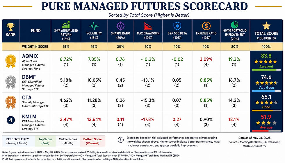
An index is a convenient yardstick but investors cannot directly invest in an index — they need a real fund, with real fees. We repeated the 75/25 test using AQMIX (AQR Managed Futures Strategy Fund — a mutual fund which launched in January 2010) instead of the SG Trend Index. That provides only 16 years of data for backtesting, nevertheless it is a real-world check. We added AQMIX in 5% steps replacing stocks, up to 50% of the portfolio.
Note: AQMIX (the institutional share class) typically requires a $5M minimum initial investment unless accessed through certain financial advisors or brokerage platforms. The retail share class (AQMNX) only has a $2,500 minimum investment but a higher expense ratio [3.09% for AQMIX and 3.39% for AQMNX]. Results using AQMNX were virtually identical to those from using AQMIX (although annual returns were higher with AQMIX compared to AQMNX due to the lower expense ratio). Data from AQMIX was used in this article.

Figure 7. The same test using a managed futures mutual fund (AQMIX), January 2010 onward. Volatility and worst loss fall steadily; the Sharpe ratio is flat across 30–40%, then declines.
AQMIX | Annual return (CAGR) | Volatility | Worst loss | Sharpe | CAGR: 2010–19 / 2020–26 |
0% | 9.36% | 12.33% | −26.22% | 0.67 | 9.00% / 9.89% |
10% | 8.76% | 10.55% | −22.43% | 0.71 | 7.98% / 9.92% |
20% | 8.11% | 8.96% | −18.63% | 0.75 | 6.95% / 9.86% |
30% | 7.44% | 7.63% | −14.88% | 0.79 | 5.91% / 9.74% |
40% | 6.72% | 6.65% | −11.87% | 0.79 | 4.86% / 9.54% |
50% | 5.98% | 6.17% | −11.24% | 0.73 | 3.80% / 9.29% |
75/25 starting portfolio with AQMIX added, since January 2010. Shaded rows are 30–40% AQMIX.
The general pattern very closely matches the SG Trend Index. Over the full 16 years, a 40% allocation to AQMIX resulted in a 46% volatility reduction, a 55% worst loss reduction, and a 28% reduction in annual return. The Sharpe ratio rose from 0.67 to 0.79 for a 30% to 40% allocation to AQMIX.
Era by era, the fund results resembled the index results but with some differences. In 2010–2019, annual return fell slightly more when using AQMIX than when using the index. In 2020–August 2026, adding AQMIX cost almost nothing in annual return reductions, while there was a more notable cost when using the index.

Figure 8. SG Trend Index (solid) versus AQMIX (dashed) in the two overlapping eras. In 2010–2019 the fund gave up somewhat more return than the index; in 2020–2026 it gave up very little.
The takeaways
The AQMIX test provides a useful real-world comparison: over its January 2010–August 2026 history, adding the fund reduced portfolio volatility and maximum drawdown, and its highest reported Sharpe ratios occurred around the 30–40% AQMIX allocation range. While the fund's results differ slightly from the SG Trend Index results, and we only have 16+ years of data for AQMIX, the impact of adding AQMIX to a portfolio is very similar to the impact from adding the SG Trend Index. The index is not directly investable, while actual funds have their own expenses, implementation choices and tracking differences. One fund's history cannot establish that other managed-futures funds will produce similar results.
Caveats
Backtests are not forecasts. Managed futures could behave differently in the future, and the 2020 and 2022 results contributed heavily in the 2020–2026 era, as did the 2000-2002 and 2007-2009 results in the first decade. As the well-known saying goes: “Past performance is no guarantee of future results”.
The index is not a fund. You cannot invest directly in the index. Real funds charge fees, can lag the index, and can differ from one another. In spite of its high fees, AQMIX still produced impressive positive impact on the portfolios in our back tests.
Monthly data and drawdown limitations. We calculate annualized volatility from monthly returns and maximum drawdown from month-end portfolio values. Monthly observations can miss intra-month peaks and troughs, so the reported maximum drawdowns may be smaller than drawdowns measured using daily data. These figures are historical estimates based on the observation frequency and should not be interpreted as limits on future losses.
Tax friction. Managed futures funds are taxed differently from stock index funds, so the choice of account type (taxable or tax-deferred/tax-free retirement) has an impact on after-tax returns.
Tracking error and Fear of Missing Out [FOMO] is real. A 30–40% allocation to managed futures is far larger than most investors hold. In 2010–2019, such a portfolio would have trailed a conventional portfolio by 2.6 to 3.5 percent a year. That is a lot to ask of anyone’s patience.
Sharpe ratio and calculation methods. Sharpe ratios from different backtesting platforms are not necessarily directly comparable because platforms may use different return frequencies, annualization conventions, and risk-free rates. In the testfol.io backtests, Sharpe ratios are calculated using daily returns and daily volatility, with CASHX or a Treasury-bill-linked rate as the risk-free benchmark. The SG Trend Index backtests were computed in a different system using monthly returns and volatility and a 0% risk-free rate. These methodological differences affect the reported Sharpe ratios. Accordingly, I compare Sharpe ratios within each set of backtests rather than treating the absolute values as directly comparable across platforms.
The bottom line
For investors who value limiting portfolio volatility and deep losses at least as much as maximizing returns, this data supports four conclusions.
First, managed futures can meaningfully reduce risk in a stock-and-bond portfolio, and the cost in annual return over 26 years was modest for the first 20% or so of managed futures.
Second, in our historical tests, allocations of roughly 30–40% to managed futures produced a favorable balance between return and measured risk for both starting portfolios. That is not a universal recommendation or a forecast. The allocation that makes sense for an individual investor depends on the existing portfolio, spending needs, tolerance for losses, and willingness to endure extended periods of underperformance. For many investors, a smaller allocation (such as 10-20% in managed futures) may provide a meaningful degree of diversification without requiring such a large departure from a conventional stock-and-bond portfolio.
Third, the benefits of adding managed futures have limits. In these tests, allocations above roughly 30–40% generally produced smaller improvements in risk at increasingly larger reductions in return, and eventually risk started to increase again. And below about 10% in managed futures, the effect is small. The allocation that makes sense depends on which risk measure matters most to the investor.
Fourth, the benefit is uneven across time periods: if you add managed futures to your portfolio there may be long time periods (like 2010-2019) when the portfolio’s returns lag behind standard benchmarks, and what matters is whether you can live with that.
This article is for educational purposes only and is not investment advice. Past performance, including hypothetical backtests, does not guarantee future results. Managed futures involve risks and are not suitable for every investor. Consider consulting a qualified financial professional.
Interested in working together? |
Author: John Macy, MBA, RICP®
John Macy is a professional financial coach and the founder of FlourishingPath Financial Coaching. With over six years of experience as a financial coach, John helps pre-retirees and retirees design resilient portfolios and income streams for their next act. Read his full story here.
Sources and notes
SG Trend Index description: Société Générale CTA index materials (PDF).
SG Trend Index 2022 performance: Hedgeweek.
SG Trend Index Data: https://curvo.eu/backtest/es/indice/sg-trend?currency=usd
Trend-following in the 2010s: AQR, “You Can’t Always Trend When You Want”; see also Institutional Investor.
AQMIX and AQMNX details: AQR fund page.
All other figures are from the author’s backtests (SG Trend Index, VTSMX, VGTSX, VBMFX; AQMIX), using monthly returns (for SG Trend Index) and month-end adjusted closing prices (for VTSMX, VGTSX, VBMFX, and AQMIX) sourced from Yahoo Finance.
Backtesting statistics for AQMIX were produced by testfol.io
Appendix
Tables Showing Summary Data for Managed Futures Allocations
75/25 starting portfolio, full period (Feb 2000–Aug 2026)
Managed futures | Stocks left | Annual return (CAGR) | Volatility | Worst loss | Sharpe |
0% | 75% | 6.98% | 11.83% | −42.01% | 0.63 |
5% | 70% | 6.95% | 11.02% | −39.02% | 0.67 |
10% | 65% | 6.92% | 10.26% | −35.90% | 0.70 |
15% | 60% | 6.87% | 9.55% | −32.66% | 0.74 |
20% | 55% | 6.80% | 8.92% | −29.28% | 0.78 |
25% | 50% | 6.73% | 8.38% | −25.77% | 0.82 |
30% | 45% | 6.64% | 7.94% | −22.19% | 0.85 |
35% | 40% | 6.54% | 7.62% | −19.12% | 0.87 |
40% | 35% | 6.43% | 7.45% | −15.95% | 0.88 |
45% | 30% | 6.31% | 7.42% | −12.70% | 0.86 |
50% | 25% | 6.17% | 7.55% | −9.97% | 0.83 |
55% | 20% | 6.03% | 7.82% | −10.67% | 0.79 |
60% | 15% | 5.87% | 8.22% | −11.36% | 0.74 |
65% | 10% | 5.70% | 8.73% | −12.05% | 0.68 |
70% | 5% | 5.52% | 9.34% | −12.74% | 0.62 |
75% | 0% | 5.32% | 10.02% | −14.52% | 0.57 |
60/40 starting portfolio, full period
Managed futures | Stocks left | Annual return (CAGR) | Volatility | Worst loss | Sharpe |
0% | 60% | 6.45% | 9.70% | −34.26% | 0.69 |
5% | 55% | 6.40% | 8.91% | −30.94% | 0.74 |
10% | 50% | 6.34% | 8.18% | −27.48% | 0.80 |
15% | 45% | 6.27% | 7.53% | −23.88% | 0.85 |
20% | 40% | 6.19% | 6.98% | −20.18% | 0.90 |
25% | 35% | 6.10% | 6.56% | −17.03% | 0.94 |
30% | 30% | 5.99% | 6.29% | −13.79% | 0.96 |
35% | 25% | 5.87% | 6.20% | −10.45% | 0.95 |
40% | 20% | 5.74% | 6.29% | −8.19% | 0.92 |
45% | 15% | 5.60% | 6.55% | −8.90% | 0.87 |
50% | 10% | 5.44% | 6.96% | −9.61% | 0.80 |
55% | 5% | 5.28% | 7.51% | −10.31% | 0.72 |
60% | 0% | 5.10% | 8.16% | −11.01% | 0.65 |
75/25 starting portfolio by era
Era | Managed futures | Annual return (CAGR) | Volatility | Worst loss | Sharpe |
2000–2009 | 0% | 2.66% | 12.71% | −42.01% | 0.27 |
10% | 3.56% | 10.86% | −35.90% | 0.38 | |
20% | 4.40% | 9.34% | −29.28% | 0.51 | |
30% | 5.17% | 8.35% | −22.19% | 0.65 | |
40% | 5.88% | 8.07% | −15.95% | 0.75 | |
50% | 6.52% | 8.58% | −9.97% | 0.78 | |
2010–2019 | 0% | 9.17% | 9.62% | −14.01% | 0.96 |
10% | 8.31% | 8.61% | −12.61% | 0.97 | |
20% | 7.44% | 7.80% | −11.20% | 0.96 | |
30% | 6.55% | 7.25% | −9.78% | 0.91 | |
40% | 5.64% | 7.02% | −9.46% | 0.82 | |
50% | 4.71% | 7.14% | −9.54% | 0.68 | |
2020–2026 | 0% | 10.35% | 13.40% | −22.77% | 0.81 |
10% | 9.95% | 11.56% | −17.70% | 0.88 | |
20% | 9.50% | 9.85% | −12.47% | 0.97 | |
30% | 9.01% | 8.34% | −9.08% | 1.08 | |
40% | 8.46% | 7.16% | −6.80% | 1.17 | |
50% | 7.88% | 6.48% | −5.88% | 1.21 |
60/40 starting portfolio by era
Era | Managed futures | Annual return (CAGR) | Volatility | Worst loss | Sharpe |
2000–2009 | 0% | 3.49% | 10.27% | −34.26% | 0.39 |
10% | 4.34% | 8.50% | −27.48% | 0.54 | |
20% | 5.13% | 7.21% | −20.18% | 0.73 | |
30% | 5.85% | 6.70% | −13.79% | 0.89 | |
40% | 6.51% | 7.12% | −8.19% | 0.92 | |
50% | 7.11% | 8.34% | −9.61% | 0.87 | |
2010–2019 | 0% | 8.12% | 7.65% | −10.44% | 1.06 |
10% | 7.25% | 6.72% | −9.00% | 1.08 | |
20% | 6.36% | 6.06% | −7.55% | 1.05 | |
30% | 5.45% | 5.78% | −7.41% | 0.95 | |
40% | 4.52% | 5.92% | −7.49% | 0.78 | |
50% | 3.57% | 6.46% | −7.95% | 0.58 | |
2020–2026 | 0% | 8.44% | 11.48% | −21.15% | 0.77 |
10% | 8.01% | 9.63% | −16.02% | 0.85 | |
20% | 7.53% | 7.92% | −10.92% | 0.96 | |
30% | 7.01% | 6.48% | −5.89% | 1.08 | |
40% | 6.44% | 5.50% | −3.97% | 1.17 | |
50% | 5.83% | 5.26% | −6.95% | 1.10 |


Comments